Linear Algebra for Machine Learning (Ch1: Vector)

Linear Algebra is a field of mathematics that could be called as the mathematics of data. It is undeniably a pillar of the field of machine learning and many recommend it as a perquisite subject to study prior to getting started in machine learning.
As per my advancement in this topic, I will post a blog here.


The fundamental building block of Linear Algebra is Vector.
So, What the vector is?
There are 3 discrete ideas about vectors, according to the prospective of  a Physics, Computer Science and Mathematics.
Physics Perception:
Vectors are arrows pointing in space having a length and direction to define it. In a plane the vector is 2 dimensional and in the space where we live in are 3 dimensional.
Computer Science Perception:
Vector is a ordered list of numbers. It could be considered as the feature of a model. We can represent the vector as a list in computer codes and theories.
A list having length 2 can be seen as 2 dimensional vector and 3 dimensional vector is a list having a length of 3.
Mathematics Perception:
Mathematics has a generalized perception of both view of the vector. Here the vector is an object having a direction and magnitude. And we also can perform arithmetic operation on them like adding two vectors and multiplying numbers to it.
[In this chapter we are going to analyze the vector addition and scalar multiplication in a deliberative manner]
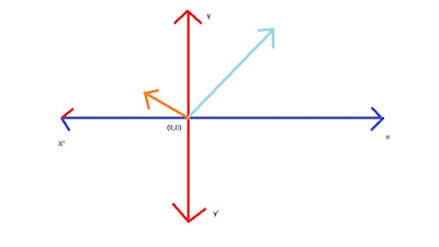
Coming to the beginning, lets consider vector is an arrow inside a coordinate system (x,y plane), where the tail is at the origin (0,0) and the arrow is at the given point. It may be different from the Physics perception (i.e. the vector can be placed anywhere in the plane), but in linear algebra the vector is rooted at the origin.

The coordinates of a vector is just a pair of numbers that is a information to travel from the origin (tail of a vector) to the tip. The first number tells us, how much to walk along the x axis and the second number instructs how much to walk in the line parallel to the y axis. The positive number says a forward or right moment and the negative number shows the backward or left moment in y and x axis direction respectively.
In 3 dimension we have

In 3 dimension we have another axis present in the coordinate system, i.e. z axis which is parallel to both x and y axis. Each vector associated with all x axis, y axis and z axis.

Vector Addition:
We can take example of a man walking 6 meters from his home and then stopped at a shop. After few minutes he again start walking in same direction for 3 meters. The total distance from current position to his home is 6+3=9. This is an example in a straight line or 1 dimension.

In the same way if we consider the queen movement in a chess board. Lets consider following two moves

1. Right up-corner move 2 : (2,2)
2. Right 2 : (0,2)

By taking the 4C as the origin (0,0) of the chess board. The Coordinate of the queen after the first movement (2,2)) will be at 6E and after the second move (0,2) the position of the queen is at 6G.
So the total movement is (2+0,2+2)=(2,4).

Scalar Multiplication:
Multiplying a number with a vector is like stretching or squeezing a vector.
Let consider a vector (2,2), that is multiplied with 2

If we have to multiply a negative no with a vector then we just have to flip around the vector and perform the operation.

 These process of stretching, squeezing and flipping of the vector is called scaling. Those numbers used for scaling a vector is called as Scalars.

Finding the optimal value of k in kNN classifier

ABSTRACT: A major issue in k-nearest neighbor classification is how to choose the optimum value of the neighbourhood parameter ‘K’. Popular cross-validation techniques often fail to guide us well in selecting k mainly due to the presence of multiple minimizers of the estimated misclassification rate. In this study we will discuss the effect of change in the value of ‘k’ on different data sets and find out the optimal value of ‘k’.

Keywords: Cross-validation; Misclassification rate; Neighbourhood parameter; Non-informative prior;

1. Introduction

The k-Nearest-Neighbors (kNN) is a non-parametric classification method, which is simple but effective in many cases. For a data record t to be classified, its k nearest neighbors are retrieved, and this forms a neighborhood of t. Majority voting among the data records in the neighborhood is usually used to decide the classification for t with or without consideration of distance-based weighting. However, to apply kNN we need to choose an appropriate value for k, and the success of classification is very much dependent on this value.

kNN has a high cost of classifying new instances. This is single-handedly due to the fact that nearly all computation takes place at classification time rather than when the training examples are first encountered. Its efficiency as being a lazy learning method without pre-modelling prohibits it from being applied to areas where dynamic classification is needed for large repository.

2. Problem Definition

The kNN method is biased by k. There are many ways of choosing the k value, but a simple one is to run the algorithm many times with different k values and choose the one with the best performance. In this study we are going to do the same.

3. Experimental Design

For the study, we have taken 4 benchmark training datasets from UCI machine learning repository i.e. Heart Disease, Dermatology, Diabetes and Haberman’s Survival to examine the changes in correctly classified instances of kNN classifier.

This chosen approach is going to be implemented on Weka tool. Weka is an open source software tool which consist of an accumulation of machine learning algorithms for data mining undertakings.

Attribute information:

	Name of the Data Set	No of	No of	Class Information
		Attributes	Instances
1	Heart Disease	13	301	{ '<50>50_1', '>50_2', '>50_3', '>50_4'}
2	Dermatology	34	360	{1,2,3,4,5,6}
3	Diabetes	8	763	{tested negative, tested positive}
4	Haberman’s Survival	4	301	{'survived 5yr','not survived 5yr'}

[Table 1: Visualization of training datasets in weka with respect to class attribute]

  

4. Results and Discussion

Experiment using the 5-fold cross validation method has been carried out to evaluate the prediction accuracy of kNN Model, and to compare the experimental results. Some information about these datasets is listed in Table 2.

Value of K	1	3	5	7	9	13
Data Set
Heart Disease	76.49	79.47	82.45	82.45	83.11	83.44
Dermatology	93.35	95.56	96.12	95.84	96.39	96.12
Diabetes	68.67	73.26	74.04	72.73	74.04	74.44
Haberman’s Survival	67.1	70.09	70.76	72.75	72.75	72.42

[Table 2: The Change in CCI with respect to the value of k observation]

In the table 2, the meaning of the title in each columns represents different values of k and rows represent the classification accuracy in different dataset. From this we can conclude that the optimum value of k purely depends upon the training dataset.

The table 3 demonstrated the comparison between the expected class value and predicted results for different data sets with their optimum ‘k’ value. As the accuracy of Heart Disease and Dermatology are very high, so they predicted the test set instances very precisely. Other two data set also performed well according to their accuracy. 

One more thing we have observed that the accuracy i.e. Correctly Classified Instances are directly proportional to the number of attributes in the training data set. A brief comparison is provided in chart 1.

5. Conclusion

The optimum K will always vary depending of your data-set. It should be as big that noises won't affect the prediction highly. And as low that one factor won't dominate another. Some claims that square root of n is a good number. But, from this study I think the best method is to try many K values and use Cross-Validation to see which K value is giving the best result.

6.  References

1. Pınar U.: HABERMAN’S SURVIVAL IN ARTIFICIAL NEURAL NETWORKS, EECS-589 İntroduction to Artificial Neural Network, (05)2014.

2. Yang S., Jian H., Ding Z., H. Zha1, and C. Lee Giles: IKNN: Informative K-Nearest Neighbor Pattern Classification, J.N. Kok et al. (Eds.): PKDD 2007, LNAI 4702, pp. 248–264, 2007.

3. Gongde G., Hui W., David B., Yaxin Bi, and Kieran G.: KNN Model-Based Approach in Classification, European Commission project ICONS, project no. IST-2001-32429.

4. Ahmad Basheer H., Mohammad Ali A., Ahmad Ali A.: Solving the Problem of the K Parameter in the KNN Classifier Using an Ensemble Learning Approach, (IJCSIS) International Journal of Computer Science and Information Security, Vol. 12, No. 8, August 2014 

Anatomy of brain

To understand how the brain computer interaction occurs, we have to know the concepts of human brain and its functionalities.

Human brain contains billions of nerve cells arranged in a particular pattern that coordinate emotion, behaviour, thought, sensation etc. Like the national highway connects all parts of the country to the capital, here in human body a very complicated highway system of nerves connects the brain to the rest of human body.

The cerebrum is the largest part of the human brain, this what we generally visualize a human brain. The outermost layer of the cerebrum is called cerebral cortex. Sometimes it also referred as grey Matter of the brain. The wrinkles and deep folds in the brain increases the surface area of the grey matter, so more information can be processed.

The cerebrum divided into two halves by a deep fissure. The sides of the brain communicate with each other through a thick tract of nerves, called the corpus callosum, at the base of fissure.

It is believed that the one side of body is controlled by the opposite side of the brain.

The hemisphere of the brain can be further divided into 4 parts.

1                     The frontal lobes :Thinking, Planning, Organizing, Problem Solving, Short term Memory

2                     The parietal lobes: Sensor

3                     The occipital lobes: Process images from eye and link to the memory

4                     The temporal lobes: process the sensor information

The cerebellum is situated below the brain at the back, and it combine the sensor information received from eye ear and muscles to coordinate the body.

The brainstem links the brain to the spinal cord. It controls many functions that are very important to life, such as heart rate, blood pressure and breathing. This area is very important fro sleep.

The core of the brain controls emotion and memories is known as Limbic system, and these structures come in pairs as each placed in each hemisphere of te brain.

Ø  The thalamus: acts like the firewall for message passed between the spinal cord and the cerebral hemisphere

Ø  The hypothalamus: controls emotion

Ø  The hippocampus: memory manager

The nervous system is all the nerves in the body, that are connect the brain with the body through the spinal cord.

Neurons have two man types of branches coming off their bodies.

1                     Dendrite: receive the incoming signals

2                     Axon: carried in the signal from nearby neuron

Inter neuron communication is very fast.

A neuron communicates with each other cells through electrical impulses, when the nerve cell is stimulated.

Within a neuron, the impulse moves to the tip of an axon and causes release of neurotransmitter chemicals that acts as messengers.

Neurotransmitters pass through the gap between two nerve cells, called Synapse and attached to receptors on the receiving cell.

This process repeats from neuron to neuron, s the impulse travels to destination.

This web based communication that allows the human to move, think, feel and communicate.

For every job and feelings there is a different web combination.

Studied from: http://www.mayoclinic.org/brain, Wikipedia, youtube

My Introduction to Brain Computer Interface

Generally we use input devices such as mouse, keyboard to give instructions to the computer. In this way, Human Computer Interaction occurs.

We know that, there are some sensors deployed on the devices that provide data to the CPU. Systematically manipulating the sensor data we communicate with the computer.

It is applicable for every machine.

As we know, human body is also a machine like computer. Where CPU is the brain, senses are the input devices and hands and feet are the output devices etc.

To give an input to the computer through the mouse, the brain first analyses the situations like “where the mouse pointer is”, “where to click” etc. by collecting the information from eyes or any other senses. Then it (brain) transmits its instruction to the hand to react. Then hand do its job.

It seems simple.

But in case of doing multiple jobs at a time, like moving the cursor (mouse) and pressing the key on keyboard, just like playing games on PC.

It became a bit difficult, because human brains are not literally meant for multitasking. Brain has to take information about many thing simultaneously like key placement, finger placement etc. to instruct both hands.

At a simple situation, just like playing the game we face such difficulties. Just imagine for the situation like space-shuttle lunching, war commanding centre, and robotic surgery etc., where each step and each millisecond counts. And a small human error can costs a million or a billion or many life.

To minimize the error and the time gap, scientists came with the concept of Brain Computer Interaction (BCI) or Brain Machine Interaction (BMI).

Where the brain directly communicate with the computer to give instructions. Here we don’t have to move our hand or leg, we just need to THINK what we want to do.

Thank you and please leave comment.

Credits : Siba Prasad Pati, Sumeet Roy